What Developers Should Know About Networks
Part One: The Physical Layer

The IEEE specification for Ethernet is over 4,000 pages long. It gets into incredibly boring minutiae: design specifications for coaxial trunk cable connectors, compliance interconnect magnitude response curves, link aggregation TLV usage rules, etc. My goal here is to omit 99.9% of those details and go for the juicy 0.1% that are relevant to anyone who wants to have a mental model of networking. If you work on any sort of networked application, my hope is that a rough model will help you feel more comfortable with what is happening further downstack.
I love computer networking. It has loads of real-world cost/benefit tradeoffs, abstractions and designs that have stood the test of time and scale, funny workarounds that got layered on top, and a rich and fascinating history that spans computer science, electrical engineering, telecommunications, information theory, and physics.
And it all comes together into something magical. We talk to people across the world instantaneously. Data flies invisibly through thin air. It’s Harry Potter-level magic, right on this planet. Thanks to exhaustive standardization, I can take my laptop from San Francisco to a village in Tanzania and the Wi-Fi will work. Yet most of us only really become aware of the network when it’s slow, or when we see a cryptic error message like ERR_NAME_NOT_RESOLVED.
The Networking Stack
The networking stack is how we maintain our sanity when talking about networks. It is a theoretical layer cake of abstractions and encapsulations that help isolate the many responsibilities and concerns of networking. In reality, there’s a lot of sophisticated dovetailing of responsibilities and blurry boundaries between the layers. Ask a network engineer how many layers there are in the networking stack, and they will give you some number between 3 and 7.
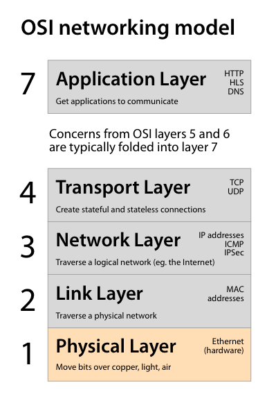
You’ll get different answers because there are several competing theoretical models used to describe the networking stack. The OSI (Open Systems Interconnection) model has 7 layers, but the Internet model has only 4 layers. Other models have five layers. But when engineers talk about “Layer 2 switching” vs. “Layer 3 switching,” they are referring to OSI layers. So, for this series, I’ll stick with those too.
At the bottom of the layer cake we have bits and cables and radio signals (layer 1) and at the top we have application protocols, like HTTP (layer 7). And the middle layers need to make a whole bunch of things possible: stateful connections, IP addresses, congestion control, routing, security, reliability, and so on.
A request for a web page moves down the layers from the browser and out onto the network. As the request moves across the internet, various devices will see it, modify its network headers, and pass it along. These devices are mostly routers and switches that operate on layers 1–3 and ignore everything else. When a response comes back it will come into the network adapter and make its way up the stack from the bottom, ending up back in the web browser.
Let’s start at the Physical Layer (layer 1)— the network’s root structure. The Physical Layer ensures that bits can move around smoothly and safely using electricity, light, or radio waves. It includes the fiber optic cables that run up and down the streets and under the oceans, the CAT-6 twisted-pair copper cables that knit their way through data centers and office parks, and the ubiquitous, invisible Wi-Fi radio signals.
While the upper layers in the stack are concerned with the information being conveyed, at the Physical Layer data is really just bits. Beyoncé or Mozart, HTML or PNG, TCP or UDP, static or streaming — it really doesn’t matter. If we can send a stream of bits reliably between two devices, a huge part of the Physical Layer’s job is done.
Specifically, we need to get data onto the wire and off of the wire (signal modulation and channel coding), notice and correct any errors that occur, and synchronize our communications. These concerns are part of the Physical Layer because they are deeply tied to the medium. For example, a particular style of digital modulation that works great on twisted-pair Ethernet would be unsuitable for Wi-Fi.
The Physical Layer determines the speed of the connection (bandwidth) and the distance a signal can travel (run length). As we move further up the stack, we will be able to abstract away the medium and communicate across the many different media that comprise the internet.
Noise Reduction
Our biggest enemy at the physical layer is noise. A given medium is only as good as the signal-to-noise ratio you can get out of it. So, let’s talk about noise reduction.
A Wi-Fi radio may be the most noisy medium in common use. It favors convenience over reliability. I can’t heat up a cup of coffee in the microwave without my Wi-Fi dropping out. It’s a miracle that Wi-Fi works at all, really. Optical fiber, on the other hand, has almost no noise at all. It’s just light.
If fiber and Wi-Fi are at two ends of the spectrum of noise, 1000BASE-T (Gigabit Ethernet) is somewhere in the middle. There’s a constant din of electromagnetic interference.
We have Alexander Graham Bell to thank for Ethernet’s first defense against noise. He found, over a century ago, that when two separate wires are twisted together as a pair, it cancels out a lot of interference and allows for a stronger signal over a longer cable length. Today, the Ethernet cables that run many of the world’s networks uses twisted pairs of copper wire.
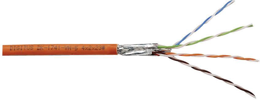
A typical twisted pair cable CC-BY-ND 2.0 Robert Webbe
The design of the cable and its connectors is crucial to noise reduction. Four pairs of wire are used to create four concurrent, bidirectional traffic lanes within the cable. Each pair has a subtly different twist rate, reducing interference between pairs.
Gigabit Ethernet adapters include a digital signal processor (DSP) that helps reduce noise. The DSP applies adaptive filtering to cancel out echo and crosstalk interference that are inevitable when you’re moving a lot of data through copper. The filtering is “adaptive” because the DSP can listen to noise patterns on the cable and effectively subtract much of it away from the signal in real time. (Adaptive noise filtering DSPs are built into everything, by the way, from mobile phones, to digital cameras, to mobile phone digital cameras.)
In addition to filtering out noise, we also need to create noise. Ethernet signals are always scrambled using a pseudorandom number generator (PRNG) on both ends of the connection. We’ve done all this work to reduce noise in our transmission, only to add noise using randomness. For power and interference and FCC compliance reasons, we never want a long string of zeroes or a long string of ones to be sent along the cable. A scrambled signal looks like white noise, and its pseudorandom data pattern allows our signal to be spread out uniformly over a range of frequencies. To be clear, this isn’t a secure PRNG, so there’s no security value in scrambling the signal at this layer. An interloper could easily guess the PRNG’s seed value and descramble the traffic on the cable.
Digital Modulation (aka line coding)
So, how do we actually get our 0’s and 1’s onto a copper Ethernet cable? That is, how do we modulate our digital bits into the analog world?
With Gigabit Ethernet, it’s complicated. So let’s rewind to the 1990s and talk about how this worked back then, when the typical Ethernet speed was 10MBits/s instead of 1Gbit/s.
On a 10BASE-T Ethernet link, there was only one traffic lane in each direction. This used two pairs of wires, one for sending (TX+ and TX-) and the other for receiving (RX+ and RX-). Messages were sent using differential voltages. The receiver measures the difference in voltage between the two receiving wires, and that difference represents a symbol. A “zero” was represented as +2.5V on the TX- wire, and -2.5V on the TX+ wire, and a “one” was +2.5V on the TX+ wire and -2.5V on the TX- wire.
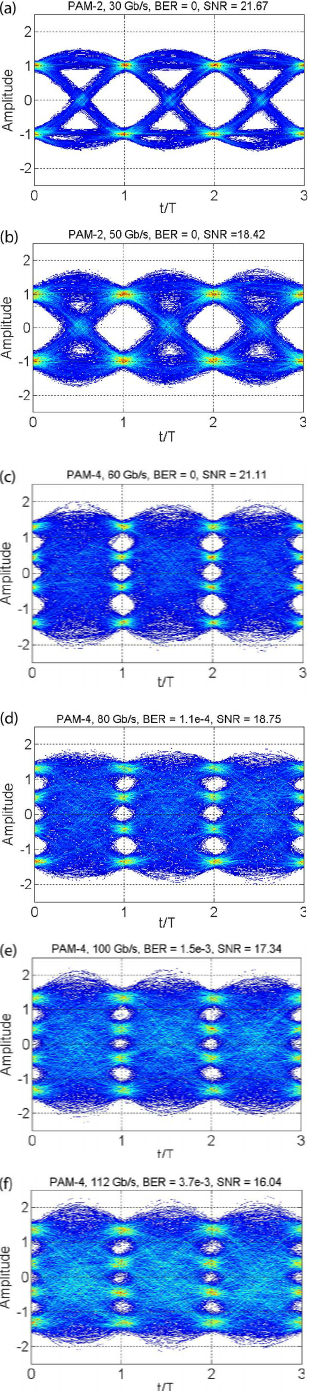
Fig 1. eye diagrams from an oscilloscope Researchgate
Using voltages that are relative to each other within each twisted pair allows Ethernet to have galvanic isolation—meaning devices don’t have to share a common ground. The same idea is still in use today with Gigabit Ethernet, except now there are five voltage levels (-2V, -1V, 0V, 1V, 2V) and there’s a more complex mapping system between bits and voltages.
We can see this in action with an eye diagram. An eye diagram (fig 1) shows how different link speeds and modulation schemes affect the signal-to-noise ratio and bit error rate. Oscilloscope probes are connected to the cable, and each diagram shows a composite of many signals over time along the wire. The amplitude is the voltage level, and the size of the white gaps (the “eyes”) gives a simple visual indicator of the signal-to-noise ratio.
Channel coding
We figured out how to design a low-noise medium and how to modulate and demodulate our data. But we can’t just send data and expect that the other end will receive it without any trouble. How can the receiving end verify that what we sent is what they received? How can we minimize the impact of noise even further? The acceptable bit error rate for Gigabit Ethernet is less than 0.00000001%, so we really can’t propagate noise up the stack from the Physical Layer.
We need a good channel coding scheme—the digital equivalent of the NATO phonetic alphabet (Alfa, Bravo, Charlie, Delta…). A good channel coding scheme will make the transmission clearer and less error-prone to the recipient.
A simple solution would be to add a parity bit for every 7-bit word being sent. A parity bit tells us whether the sum of the bits in a word are even or odd. So, if we’re trying to send the 7-bit word 0101010, we might send 10101010, adding a 1 at the beginning to indicate that the sum of all the other 1s is odd.
This would detect some errors, but it would require us to ask for retransmission when errors occur. To stop everything and ask, “What did you just say?!” is annoying. So instead of merely detecting errors, we’d like a coding scheme that can detect and correct for the most common errors.
This is where error correcting codes (ECCs) come in. The simple idea is to add enough redundancy to the signal to stay below our acceptable bit error rate.
Here’s a very simple “rate 1/3” error correcting code, in which three bits (a “symbol”) are sent in order to represent a single bit of data. A zero from the sender becomes 000 on the wire, and a one becomes 111. If 000 was sent, and the recipient heard 001, they can recover a “likely 0.” If 111 was sent and the recipient heard 011, that’s a “likely 1.” And if a 111 was sent and a 111 was received, then it’s an error-free 1.
The amount of redundancy we need will greatly depend on the medium. Going from the Earth’s surface to a Mars rover is the ultimate bad wireless connection. The signal from Earth fades as it travels through the atmosphere and into deep space, and the signal-to-noise ratio drops gradually. Once it reaches Mars it’s very faint. Furthermore, communication takes 14 minutes each way. If we have to ask for retransmission of data, we’ll be waiting 28 minutes. So, we need a lot of redundancy. With an error correcting code, we might transmit a 100 bit symbol in order to represent a single bit of data. This is a “rate 1/100” code. Not very efficient, but necessary for deep space communication.

Fig 2. A map of Hamming Distances. How many bits must be flipped to get from one binary value to another? The color for each (x,y) point represents the Hamming Distance between x and y. Darker colors represent fewer bit flips.
Coming back to Earth, let’s improve upon our repetitive rate 1/3 code. Rather than simply repeating one input bit several times, more sophisticated ECCs add redundancy to longer blocks of input bits. A classic “block code” is the Hamming(7,4) code, invented in 1950 by coding theorist Richard Hamming. In Hamming(7,4), a four bit input is cleverly mapped to a 7 bit output that is spread as far apart as possible from other possible output values in terms of their Hamming distances (see Fig 2). In other words, the 7 bit outputs are more distinctive from each other than the 4 bit inputs, in the same way that saying “Bravo” and “Delta” is more distinctive than saying “Bee” and “Dee” to represent the letters B and D.
Hamming(7,4) is a rate 4/7 code, so it provides a better transfer rate compared to a rate 1/3 code. But, it still doesn’t get us what we need to handle the latest Ethernet or Wi-Fi standard.
Maximizing Bandwidth
We’re looking to cheaply move data as quickly as possible, for reasons that are obvious to anyone who has polished off an entire bucket of buttery popcorn while watching the loading spinner for the 4K HDR version of “Moana.”
Step back for a second and notice that we continue to improve bandwidth over the years even though the medium stays mostly the same. How does Wi-Fi keep getting faster, when the underlying physical constraints aren’t changing? How can we run 10Gbits/s over roughly the same copper cables that in the 1990s could only handle 10Mbits/s?
We’re better at coding and modulation than we used to be. We’re better at manufacturing cables with tighter tolerances very cheaply. Most importantly, Moore’s Law has made it possible for cheap networking hardware to run more complex coding schemes. Hamming(7,4) was great in the 1950s, but for 10 Gigabit Ethernet, the decoding and demodulating process is an NP-complete problem solved using an AI inference algorithm called belief propagation. Running that algorithm on 90s hardware wouldn’t have been worthwhile.
Gigabit Ethernet has a symbol rate of 125,000,000 symbols per second. That’s a symbol every 8ns. What’s a symbol? It’s 12 bits (two bits per wire * 4 wires) that, after demodulation and decoding, represents 8 bits worth of data.
125M symbols/sec/pair * (2 bits * 4 pairs of wire)/symbol = 1000 Mbits/sec in both directions.
Now, you might be wondering how we can move 1,000 Mbits/s in both directions at the same time?
Here’s how that works. For a given 8ns window, imagine host A wants to send a voltage differential of +1V on one of the twisted pairs. Host A sets the voltages of the pair to +0.5V/-0.5V respectively. Meanwhile, at the other end of the cable, host B wants to send a differential of +2V. So, host B sets the voltages to +1V/-1V.
Now, both of them sample the voltage differential on the wire. Because the voltages are additive, both ends will see +1.5V/-1.5V. They will sample, in other words, a +3V differential. Host A can safely subtract out the +1V differential it sent, and interpret what’s left as a +2V signal sent from host B. And host B can safely cancel out the +2V it sent, and read the +1V signal from host A.
Synchronization
Another concern is synchronization. Both ends of the connection need to know when to sample the voltage on the wire. The best place to sample the voltage is right in the middle of the 8ns window for a given symbol. Ethernet uses a technique called clock recovery in order to get in sync. Clock recovery analyzes the frequency and phase of an incoming signal and figures out where one symbol starts and end without explicitly needing to be told. That is, it “recovers” the clock from the signal, using a process that’s a bit like tuning an analog radio until the station comes in clearly.
There’s so much more to the Physical Layer. We didn’t talk about flow control and link autonegotiation. We didn’t talk about the complexities of Wi-Fi communications (what is a radio, really?). We didn’t even talk about physical network topologies. But my hope is that we covered the Physical Layer’s basic responsibilities. The next layer up is the Link Layer—layer 2—which allows us to establish a local network using physical MAC addresses. Layer 2 is still strongly tied to the medium and doesn’t care about the meaning of the data. But, as we move up the stack, the meaning of the data starts to emerge from the primordial soup of bits will become a lot more important.
Thanks to Siobhán Cronin and Xiaowei Wang for proofreading this piece.